Replication Package For Paper: Learning CNN-Encoded Propositions of Action Sequence-based Robotic Programs from Few Demonstrations
View on Github
Code
We implement the code of this project, which can be found here.
Video
capNet
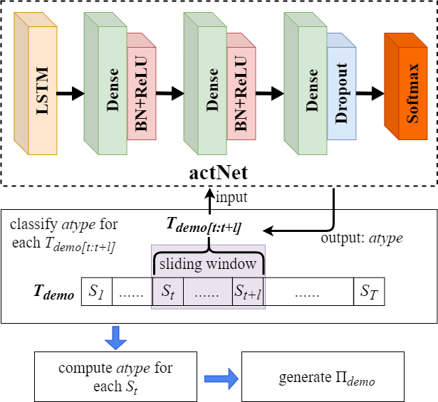
The input to the capNet is a 200×65 trajectory fragment. The first layer consists of two stacking LSTMs which is bidirectional and contain 128 hidden states. It is followed by two fully-connected network blocks, each is composed of a dense layer, a batch normalization layer and a ReLU activation function layer. The hidden sizes are 256×128 and 128×64 respectively. The output layer consists of a 64×4 dense layer followed by a dropout layer with p = 0.5. The multiple classification result is generated by a softmax layer. During training the capNet, the Batch size is 256 and learning rate is 0.0003.
baseNet and propNet
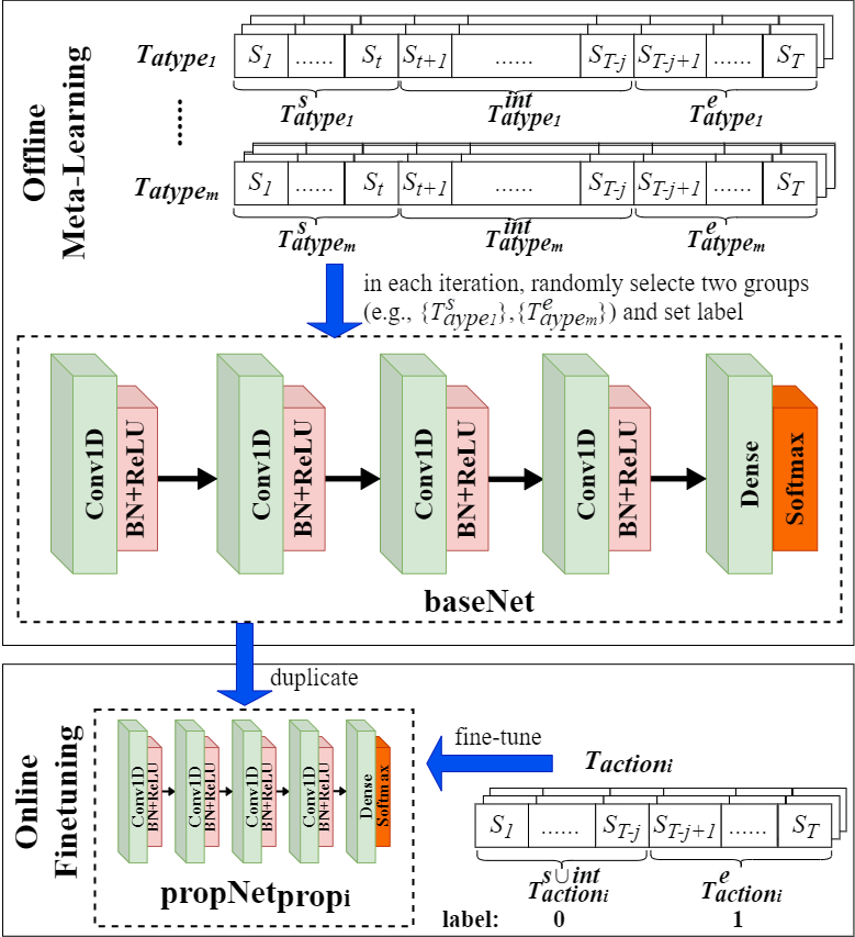
The input to the baseNet or propNet is a 50×65 trajectory action states. The basic block is composed of a convolutional layer, followed by a batch normalization layer, a ReLU activation function layer and a max pooling layer with kernel size 2. The detail is shown as following.
| layer | filter | stride | padding |
|---|---|---|---|
| 1 | 128×50×1 | 1 | 1 |
| 2 | 64×64×3 | 1 | 1 |
| 3 | 64×32×3 | 1 | 1 |
| 4 | 32×32×3 | 1 | 1 |
The output layer consists of a 64×2 dense layer and a softmax layer.
Case Study
Among the set of actions, we design a pick-and-place task. Suppose there are two tables, e.g., TableA and TableB in the simulation environment. TableA is outside a room and there is a cube on the table. TableB is inside the room. The Fetch robot is first guided to move close to TableA and then to pick up the cube. After catching the cube, the robot is guided to move to TableB and finally put the cube on the table. We perform demonstrations five times from the viewpoint of an end user.
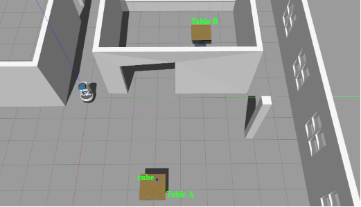
Figure: Scenario of the Task
Robot and Scenario
We present the implementation of the approach on a Fetch robot in a simulation environment. Fetch robot is mainly equipped with a mobile base and a robotic arm. The mobile base is made of two hub motors and four casters, while the arm is a seven-degree-of-freedom arm with a gripper. The actions of a Fetch used in the case study are listed in table below.
Table: Actions of Fetch used in the case study
| Action Type | Description | ROS API |
|---|---|---|
| move | The robot moves to a target by the mobile base and the arm is free. | move_base(target) |
| transport | The robot moves to a target by the mobile base while keeping the arm holding an object | move_base(target) |
| pick | The robot grabs a target object without body moving. | pick(target) |
| place | The robot puts the object held by the arm onto a target without body moving. | place(target) |
We implement the approach in a Gazebo9 simulation environment, which is high-fidelity and offers the ability to accurately and efficiently simulate populations of robots in complex indoor and outdoor environments. The execution of the actions in the simulation environment shows uncertainty due to the physics engine or the probability-based algorithms. For example, an object slips away from the gripper of a robot, or a robot follows different moving paths by the SLAM navigation algorithm. The feature increases the value of our approach since the robot behavior in the simulation environment can reflect similar variability as in the real environment with real physical hardware.
The states of the trajectories related to the robot features and the environment features can be obtained by subscribing to ROS topics. One is the joint_states topic which provides 13 joints of the robot features including the arm and the mobile base. They are
l_wheel_joint, r_wheel_joint, torso_lift_joint, bellows_joint, shoulder_pan_joint, shoulder_lift_joint, upperarm_roll_joint, elbow_flex_joint, forearm_roll_joint, wrist_flex_joint, wrist_roll_joint, l_gripper_finger_joint, r_gripper_finger_joint.
Each joint has 3 properties including position, velocity and effort. There are 3×13 joint features from fetch itself. The other is the /gazebo/model_states topic which provides 13 features associated with the position and the orientation of the robot and the cube as well. They are
fetch_pose_position_x, fetch_pose_position_y, fetch_pose_position_z, fetch_pose_orientation_x, fetch_pose_orientation_y, fetch_pose_orientation_z, fetch_pose_orientation_w, fetch_twist_linear_x, fetch_twist_linear_y, fetch_twist_linear_z, fetch_twist_angular_x, fetch_twist_angular_y, fetch_twist_angular_z.
There are 13+13 joint features from Gazebo. Thus, a state vector is composed of total 65 features. The state vectors of a trajectory are sampled with a 100Hz frequency.
Dataset
- traj_action: a large training set of robot’s action execution. This is a serialized dictionary dataset with four keys: “move”, “pick_cube”, “transport” and “place_cube”. The value of each key contains a list of trajectories for an action.
- traj_demonstration: a set of trajectories by executing the task. This is a serialized list dataset. Each element in the list is a dictionary object with four keys: “move”, “pick_cube”, “transport” and “place_cube”. The value of each key is a trajectory of an action.
Offline Training
We train the capNet based on the data set obtained from executing the four actions randomly. For example, to make the robot move around in a space, and to make the robot pick a cube which is placed in different positions on a table. We execute each action more than one thousand times and obtain the data set containing more than 4,000 trajectories. The training lasts for 50,000 epochs. Each epoch contains 10 batch data and each batch data is selected when assembling a task. We construct a meta-learner to help train the baseNet. The meta-learner manages the weights of the baseNet. In each epoch, it computes the gradients by training the tasks each by five gradient update steps. The weights of the baseNet are updated by backpropogation from the meta-learner after accumulating the loss of all the tasks. We use meta-learning to train the baseNet. The training of baseNet lasts for 50,000 epochs. propNetpropi is learned by fine-tuning on baseNet. The training for the capNet and the baseNet is conducted on a machine with an AMD Ryzen 9 3950X processor and an RTX3090 GPU running with 128 GB RAM.
Action Segmentation
We set a sliding window of length 200. Each trajectory is input to the capNet to compute the likelihood of the action label of each fragment, as presented in the figure below.
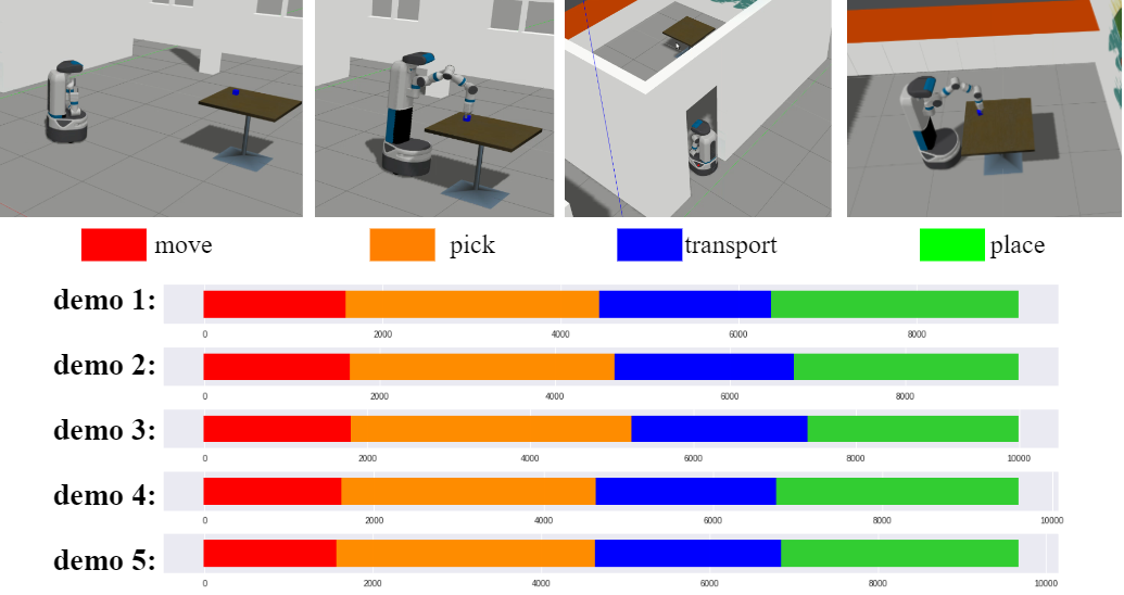
Figure: Action segmentation of the 5 demonstrations
The sequences of the five demonstration trajectories are largely the same with the task scenario. The Πtask is formulated as
propNet learning
The propNet related to the four symbols (i.e., prop1 to prop4) in the Πtask is trained subsequently. For example to train the propNetpropi for propi, we collect the trajectory fragments corresponding to the first action from the five demonstration trajectories, i.e., {Tmove1}. The fragment of the last 150 state vectors covering the end stage of the trajectory is labeled 1 and the remaining fragment is labeled 0. The propNetpropi is finetuned by a 15-step gradient descent.
Testing
We test the generated robotic program by proposing a new request but under a slightly changed environment setting. We ask the robot to pick up a cube on TableA but located in a different position from the demonstrations, and then to transport and place the cube on TableB which is in another position in the room. The request is realized by customizing the parameters of the action APIs, and thus the actions can be executed as expected. For example, the position of TableB can be obtained directly from the simulation environment. The position is specified as the actual parameter of the API, i.e., the parameter target of move_base.
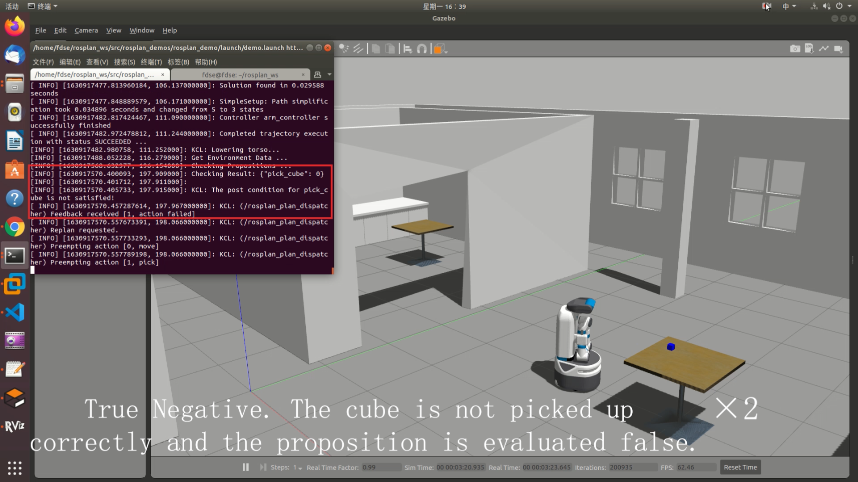
ROSPlan ingests the PDDL program and produces a four-step plan which is composed of the sequence of actions, i.e., ⟨move1, pick1, transport1, place1⟩. The TaskDispatching module manages the plan execution. When a proposition is specified in the LaunchFile, the dispatching module invokes the corresponding sensing implementation to determine whether to execute the next action by evaluating the propNet.
Experiments
- TP (true positive) represents the correct evaluation of a proposition (i.e., evaluate the truth value) to an action which is completed correctly
- TN (true negative) represents the correct evaluation of a proposition (i.e., evaluate the false value) to an action which is executed abnormally
- FP (false positive) represents the incorrect evaluation of a proposition (i.e., evaluate the false value) to an action completed correctly.
- FN (false negative) represents the incorrect evaluation of a proposition (i.e., evaluate the truth value) to an action executed abnormally.
- cnt represents the total count of proposition evaluation performed during the program execution in an experiment, the accuracy is calculated by #TP+#TN/cnt, where # means the count of the verdict.
- SeR is short for stationary-environmental request. VeR is short for variable-environmental request.
- #ES represents the count of the success during the executions. #EF represents the count of the failure.
General Accuracy
Table: Accuracy of proposition verdict of different approaches
| cnt | #TP | #TN | #FP | #FN | Accuracy | #ES | #EF | ||
|---|---|---|---|---|---|---|---|---|---|
| Baseline (5) | SeR | 137 | 95 | 12 | 30 | 0 | 78.0% | 2 | 14 |
| VeR | 79 | 29 | 3 | 47 | 0 | 40.5% | 0 | 3 | |
| Baseline (100) | SeR | 182 | 153 | 12 | 10 | 7 | 90.7% | 21 | 12 |
| VeR | 78 | 32 | 6 | 40 | 0 | 48.7% | 4 | 6 | |
| BASENET | SeR | 121 | 71 | 5 | 42 | 3 | 62.8% | 0 | 5 |
| VeR | 80 | 30 | 8 | 39 | 3 | 47.5% | 0 | 8 | |
| Ours (5) | SeR | 152 | 130 | 8 | 8 | 6 | 90.8% | 28 | 8 |
| VeR | 151 | 120 | 11 | 15 | 5 | 86.8% | 19 | 11 |
This Table shows the comparision between our method and baseline. Each method is evaluated in both SeR and VeR. We uses the robotic program which is learned and generated from five demonstrations. The experiments is executed for 50 times.
Impact of the Number of Demonstrations
Table: Accuracy of evaluating propositions for SeR under different demonstration counts
| #demonstration | cnt | #TP | #TN | #FP | #FN | Accuracy | #ES | #EF |
| 1 | 140 | 100 | 13 | 19 | 8 | 80.7% | 10 | 13 |
| 5 | 152 | 130 | 8 | 8 | 6 | 90.8% | 28 | 8 |
| 10 | 169 | 148 | 11 | 10 | 0 | 94.1% | 29 | 11 |
| 20 | 159 | 136 | 15 | 4 | 4 | 95.0% | 27 | 15 |
This table evaluates the impact of the number of demonstrations on our approach. To this end, we learn from 1, 5, 10 and 20 demonstrations in SeR. The experiments is executed for 50 times.
Generalization in extended scenario
Table: Accuracy of evaluating propositions reused in the eight-step task
| #demonstration | cnt | #TP | #TN | #FP | #FN | Accuracy | #ES | #EF |
| 5 | 258 | 213 | 15 | 14 | 17 | 88.0% | 4 | 15 |
This experiment aims to evaluate the generalization of our approach when reusing propositions learned from a basic scenario in a more complex scenario.
We retain the networks learned in the four-step task by 5 demonstrations. Then, an eight-step Πtask can be assembled as
The task is executed for 50 times in SeR setting. The accuracy for evaluating propositions is listed in Table.